Mechanistic Interpretability 1：Multi-Query Associative Recall

本文是对于 Zoology 及其前作 Hyena 架构的整理。这两篇论文均在 Hazy Research 上有一份报告，以及相应的正式论文。Zoology 至今应该仍然是对于 recall 问题的机制可解释性讨论得比较完全的文章之一，而且有很多值得思考的理论结论，所以写一篇来整理一下。

架构

在正文之前，有必要提到，这两篇论文都是基于长卷积模型的范畴讨论的，而不是线性模型的范围。对于长卷积模型的定义，在 Hyena 的论文 2.1 节前后提到。简单来说，长卷积模型的序列混合器（token mixer）是对于输入序列的一维线性（非循环）卷积，即

$y_{t}=(h*u)_{t}=\sum_{n=0}^{L-1}h_{t-n}u_{n}.$

其中假设 filter $h$ 具有负下标，如果没有则截断为 0。对于 attention 而言，序列混合为 $y=Au$，其中$A\in \mathbb{R}^{T\times T}$ 为注意力分数矩阵。长卷积模型也有类似的表示（实际上所有亚二次的架构都能够有这种形式的表示），即其向量形式

$(h*u) = \begin{pmatrix} h_{0} & h_{-1} & \ldots & h_{-L+1} \\ h_{1} & h_{0} & \ldots & h_{-L+2} \\ \vdots & \vdots & \vdots & \vdots \\ h_{L-1} & h_{L-2} & \cdots & h_{0} \end{pmatrix} \begin{pmatrix} u_1 \\ \vdots \\ u_{L-1} \end{pmatrix}$

其中的等效注意力矩阵是一个 Toeplitz 矩阵，或称常对角矩阵。对比之下，attention 的注意力矩阵完全是由输入数据控制生成的，即 data-control/data-dependent，长卷积模型的注意力矩阵完全由参数决定，与输入无关。Zoology 认为正是常对角在 pattern 上相对 attention map 的受限性导致了 recall 能力的不完全，并且实际上通过对输入数据的依赖来破坏这一模式，从而获得更好的 recall 能力。

需要注意的是，显式卷积模型之所以成为亚二次模型完全依赖于 FFT 来达到 $\mathcal{O}(N\log N)$ 的复杂度，它不能得到线性的复杂度。现代的基于 state space 的架构确实具有卷积的形式，并且通过展开为类似卷积的形式进行并行，但应该说，线性架构是长卷积架构的子类（是吗？有待验证。当然如果引入 data-dependent 的成分就不严格是了）。如果要达到全局注意力，显式卷积需要参数化与序列长度有关的 filter，当然像传统的 CNN 一样局部注意就不需要了。隐式卷积的目标是解耦参数量与 filter 的大小，即参数化一个 $\gamma_\theta$，从中获得 filter 各个地方的值 $h_t=\gamma_\theta(t)$。SSM 就是隐式参数化的一种形式，其通过状态转移矩阵参数化 filter，forward 的过程就是在执行一个参数化的卷积。这里指的依然是 data-independent 的情形，即状态转移矩阵与当前步的输入无关。

数学记号

Zoology 这篇文章很多的主要结论都在附录里面，而且有一些（好像不是那么常见的）数学记号。

第一个是非循环卷积和循环卷积的多项式表示。这一部分是根据 Gemini 2.5 的推理整理的。

The document explains how vector convolutions can be interpreted using polynomial multiplication. Let’s break down the two formulas presented in Appendix H.1.1 under “Polynomial Notation”.

Given two vectors, u and v, of length n:

• $u=[u_0, u_1, ..., u_{n-1}]$

• $v=[v_0, v_1, ..., v_{n-1}]$

We first convert these vectors into polynomials using the poly() mapping defined as $poly(w)=\sum_{i=0}^{n-1}w[i]X^i$.

So,

\begin{aligned}
u(X)&=u_0​+u_1​X+…+u_{n−1}​X^{n−1} \\
v(X)&=v_0​+v_1​X+…+v_{n−1}​X^{n−1}
\end{aligned}

The coeff() function then converts a polynomial back to a vector of its coefficients, where the $i$-th element of the vector is the coefficient of $X^i$ in the polynomial.

1. Linear Convolution: $u*v=\text{coeff}(u(X)\cdot v(X)(\text{mod}\;X^n))$

This formula describes how to obtain the linear convolution of two vectors, resulting in a vector of length n.

• u(X)⋅v(X): First, multiply the two polynomials $u(X)$ and $v(X)$. The resulting polynomial, let’s call it $P(X)$, can have a degree up to 2n−2.

• $\text{mod}\;X^n$: Next, take this product polynomial $P(X)$ modulo $X^n$. This operation effectively truncates the polynomial $P(X)$, keeping only the terms with powers of $X$ less than $n$. In other words, all terms $X^n,X^{n+1},...,X^{2n-2}$ and their coefficients are discarded. The result is a polynomial of degree at most n−1.

• coeff(…): Finally, extract the coefficients of this resulting polynomial to form the vector u∗v. This vector will have n elements, corresponding to the coefficients of $X^0,X^1,...,X^{n-1}$.

This corresponds to a specific type of linear convolution where the output sequence has the same length as the input sequences.

2. Cyclic Convolution: $u\otimes v=\text{coeff}(u(X)\cdot v(X)(\text{mod}\;X^n-1))$

This formula describes how to obtain the cyclic convolution of two vectors, also resulting in a vector of length $n$.

• u(X)⋅v(X): Again, start by multiplying the two polynomials $u(X)$ and $v(X)$ to get $P(X)$.

• $\text{mod}\;X^n-1$: This is the key difference. Taking the product polynomial $P(X)$ modulo $(X^n-1)$ means that any power of $X$ equal to or greater than $n$ “wraps around”. Specifically, $X^n \equiv 1 (\text{mod}\quad X^n-1)$, $X^{n+1} \equiv X (\text{mod}\quad X^n-1)$, and so on. For any term $X^k$ where $k \ge n$, it can be rewritten as $X^{k \quad\text{mod}\quad n}$. The coefficients of these “wrapped” terms are added to the coefficients of the corresponding lower-degree terms. The resulting polynomial will have a degree at most $n-1$.

• coeff(…): Extract the coefficients of this polynomial to form the vector $u\otimes v$. This vector will have $n$ elements.

Example

Let $n=3$, and consider the vectors:

• $u = [1, 2, 3]$

• $v = [4, 5, 6]$

Their polynomial representations are:

• $u(X) = 1 + 2X + 3X^2$

• $v(X) = 4 + 5X + 6X^2$

Polynomial Product $P(X) = u(X) \cdot v(X)$:

\begin{align} P(X) &= (1 + 2X + 3X^2)(4 + 5X + 6X^2) \\ &= 1(4 + 5X + 6X^2) + 2X(4 + 5X + 6X^2) + 3X^2(4 + 5X + 6X^2) \\ &= (4 + 5X + 6X^2) + (8X + 10X^2 + 12X^3) + (12X^2 + 15X^3 + 18X^4) \\ &= 4 + (5+8)X + (6+10+12)X^2 + (12+15)X^3 + 18X^4 \\ &= 4 + 13X + 28X^2 + 27X^3 + 18X^4 \end{align}

1. Linear Convolution Example:

$u*v = \text{coeff}(P(X) \text{mod}{X^3})$

\begin{align*} P(X) \pmod{X^3} &= (4 + 13X + 28X^2 + 27X^3 + 18X^4) \pmod{X^3} \\ &= 4 + 13X + 28X^2 \end{align*}

So, $u*v = \text{coeff}(4 + 13X + 28X^2) = [4, 13, 28]$.

2. Cyclic Convolution Example:

$u \otimes v = \text{coeff}(P(X) \text{mod}{X^3 - 1})$

$P(X) = 4 + 13X + 28X^2 + 27X^3 + 18X^4$

Modulo $(X^3 - 1)$, we have $X^3 \equiv 1$. Therefore:

$X^4 = X \cdot X^3 \equiv X \cdot 1 = X$.

Substituting these into $P(X)$:

\begin{align*} P(X) \pmod{X^3-1} &= 4 + 13X + 28X^2 + 27(1) + 18(X) \\ &= (4+27) + (13+18)X + 28X^2 \\ &= 31 + 31X + 28X^2 \end{align*}

So, $u \otimes v = \text{coeff}(31 + 31X + 28X^2) = [31, 31, 28]$.

These polynomial interpretations are foundational for understanding how operations like convolutions, which are common in sequence modeling, can be analyzed and implemented, particularly in relation to structures like FFTs (Fast Fourier Transforms) mentioned elsewhere in the document.

另一个记号是 $[d]:=\{1,2,3,...,d\}$。附录中的很多内容还涉及代数电路（arithmetic circuit）的内容，定义和计算图基本是一样的。

Recall with Attention / Data-Independent Convolution

Zoology 在 HazyResearch 上的文章给了比较直观的解释，部分细节在论文的 Appendix H.7.2 中。Attention 来进行 recall 的机制实际上就是移位-匹配，由前后两层 attention 组成，在 Anthropic 的文章中称为 Induction Head。第一层中，attention 借助位置编码（比较容易分析的形式是 ALiBi）形成常对角的模式，将前一个 token 与后一个 token 进行混合，形成如图的模式。目的是为了混合 key 和 value。

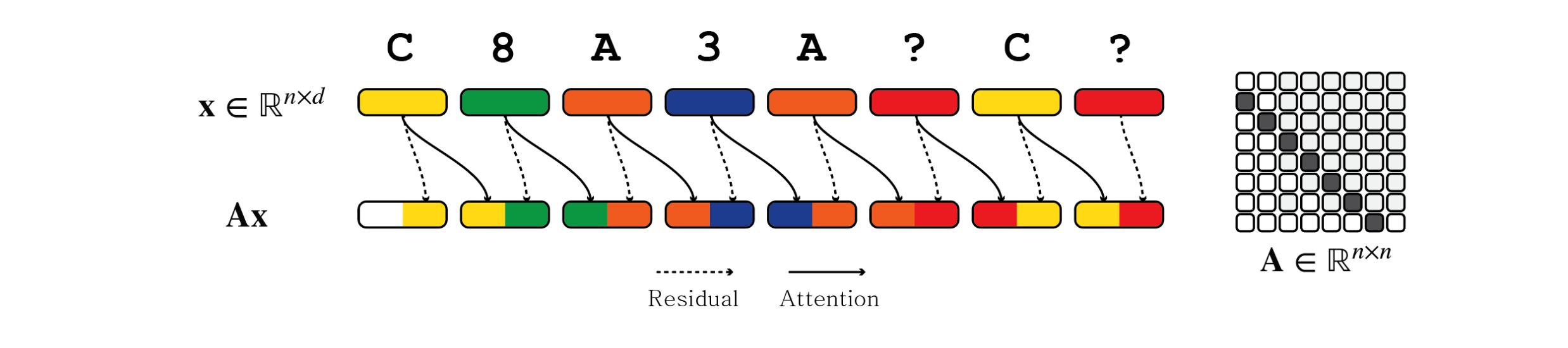
第二层将当前的 query 与 所有的 key 进行 attention 计算，从而知道匹配的位置。此时 key 已经混合了 value 的信息，因此就可以把 value 的信息直接抽取出来，直接搬到需要的位置。下图的 A 与 3、C 与 8 为 attention 选择的匹配对。

这个图实际上有一些误导性，Appendix H.7.2 说得更详细一些。attention 是没有把一个 token 的前一半 dimension 和另一个 token 的后一半 dimension 接在一起的能力的，这里假设了 query、key、value 占据不同的 dimension，互不相交。

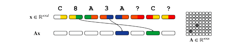
对于长卷积模型而言，注意力矩阵约束为常对角形式，因此它无法完成第二层中的操作。在常对角的约束下，$Ax$ 的结果不能对不同位置的 token 产生不同距离的位移，只能对整个句子形成统一的移动。

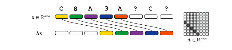
因此，卷积唯一的选择是利用 dimension 的切割，在不同的 dimension 上应用不同的位移，从而把一个 token 之前的全部上下文——而不是选择性地将 query-key 最匹配的 token——压缩到一个 token 中，然后进行匹配。

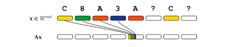
所以，长卷积模型解决 recall 问题的方式与 attention 的两层结构是不一样的。第一层中，长卷积需要将上下文压缩到单个 token 中，并找到匹配的 key 的位置；第二层中，再找出他后面的 value 是谁（shift）。整体上，卷积模型是 find-and-shift，attention 是 shift-and-find。此外，很明显 dimension 在长卷积模型中需要随着 recall 的距离增长而增长。后续引入 data-dependent 实际上解决的是这个 dimension 与 recall 距离相关的问题。

Multi-token Key-Value Pair / Fuzzy Recall

这是我个人对此的扩展。这里实际上还涉及到一个扩展的问题，如果 key 或者 value 的长度超过 1 个 token 怎么办？一个比较反直觉的结论是，attention 本身应该没有更好地处理 multi-token key 的能力。即使在多层的 attention 中，考虑最后一层，我们最终还是要用某个 query 和之前的历史比较，发现他与之前的某个 key 很像，最后取出它后续的 value。问题在于，这里的 query 本身只有一个 token。这意味着必须将 multi-token query 的信息压缩到一个 token 中才能做这件事。这件事看上去很简单，因为这就是一个卷积的事情，但 attention 本身并没有这样的能力。在上文 attention 构造的第一层中，我们实际上做了类似的事情，此时我们就不是依赖 attention 本身完成的，而是依赖 ALiBi 位置编码完成的。attention 本身没有形成局部 pattern 的能力，这使得外加卷积或者位置编码对 attention 的能力至关重要，multi-token attention 和 Physics of Language Models: Part 4.1 实际上就是在做这件事情。回到 multi-token recall 任务上来，实际上不管是 attention 还是亚二次模型都依赖于外置卷积或者位置编码来实现这件事情。这个任务的扩展暂时与 token mixer 机制本身的优劣无关。

Recall with Data-Dependent Convolution

Zoology 的架构建立在 BaseConv 上，即

$y = (u \cdot W^{l} + b_{1}^{l}) \odot (h^{l} * u + b_{2}^{l})$

也就是一个 Linear 和一个长卷积 gating 之后的结果。Data-Dependent 相关的证明没有在 HazyResearch 的网页上，见于 Appendix H.8.2。论大致思路，就是将 $h^l$ 变得和输入相关。论文使用自相关（autocorrelation）来构造 $h^l$ 。所谓自相关定义为序列 $u$ 和自身倒序的非循环卷积，实际上自相关的输出 $u'$ 中，$u'[n-1-k]$ 代表了序列 $u$ 向前移动 $k$ 位之后形成的序列和原始序列的点积，算的是 $u$ 和自身移位的点积相似度。对于一个 recall 任务，序列位移之后总会有 query 和 key 匹配上的时候，此时点积相似度应该是高的。于是假定某个函数能够给出基于自相关的导致前 $t$ 大的相似度的移位，这 $t$ 个移位实际上就是 query 到匹配的 key 的距离。

然后根据这个构造出卷积核即可。根据 $[1,2,3,4]*[0,1,0,0]=[0,1,2,3]$ 这样的性质，卷积核可以拿来进行位移。基于这一点和 gating 就可以进行匹配了。后续证略。

这实际上是一个非常理论化的证明，因为这个 Data-Dependent 的构造基本上是开了上帝视角。而且计算上也很难算得上高效，自相关本身就需要一个全局的长卷积。Zoology 最后也还是选择了 hybrid 架构。另外，自相关本身也不是匹配的最佳标准，它对比事实标准（文中的 Programmatic Filters）还是差了挺多的。

These input-dependent filters cannot easily be made to satisfy causality and using an $O(N \log N)$ filter per gap could be expensive if each gap applies only to a small number of bigrams. A simpler and perhaps more efficient way to solve the problem would be to introduce a small amount of attention to an otherwise BaseConv model [Fu et al., 2023a].